A user-guide for the GRISLI (Grenoble ice sheet and land ice) model at U. Bourgogne. A 3D ice-sheet model designed for deep-time, large-scale investigations.

This page is not intended to replace the official GRISLI user guide, but rather to provide additional / alternative material.

Updated model versions are now available here for instance. This tutorial refers to the version used by e.g. Pohl et al. (2016) or Ladant et al. (2014).

Information on the CCUB cluster can be found here.

Although the tutorial is built with many sections for readibility, I suggest progressing linearly since knowhow acquired in section n will sometimes be useful for section n+1.

Tutorial status: this page is finished, but the tutorial has never been tested yet. Happy to have feedbacks, and to revise and add content.

Introduction

This tutorial describes how to run the GRISLI (Grenoble ice sheet and land ice) model (Ritz, 2001) on the linux cluster of Univ. Bourgogne (CCUB, Dijon). It should be easy to adapt to other clusters.

This tutorial shows how to use the model in a simple way, by forcing the model with climatic boundary conditions (precipitations and surface air temperature) derived from the atmospheric general circulation model LMDZ, using a standard, large model grid of resolution 40 km × 40 km centered over the South Pole. Ladant et al. (2014) developed an asynchronous coupling method permitting to account for the feedbacks of the ice sheet on global climate (also used by Pohl et al. (2016)); this more sophisticated setup is not described here. The documentation may be updated later upon request. As for now, the experimental setup desribed in this tutorial only permits to investigate glacial inception a-la Ladant et al. (2016); it cannot be used to quantify climate-ice-sheet equilibria (For a comparison, compare Figs. 2 and 3 of Pohl et al. (2016)).

Please note that the GRISLI source code is not freely available.

Requirements

Before starting anything, you need to correctly configure your environment by loading the appropriate modules:

module purge
module load netcdf/4.5.0/intel/2018
module load intel/2018
module load cdo
module load nco
module load python/3.6

For comparison, here should be the result of the module list command:

Currently Loaded Modulefiles:
 1) netcdf/4.5.0/intel/2018   3) cdo/1.9.2/intel/2018   5) python/3.6/intel/2019
 2) intel/2018                4) nco/4.7.7/intel/2018

Remark: At some point, following cluster module updates, we will probably have to change some modules. Ideally, we’ll also have to check that results are identical.

Installing and compiling

Download the model source code plus useful files from here. Then, uncompress the directory on your work /work/crct/zz9999zz (replace zz9999zz with your CCUB login) (using unzip GRISLI.zip). As for now, the model source code is not freely available; this is why the .zip archive is password-protected. Then, enter the model directory cd GRISLI/GRISLI-version8-svn.
On the CCUB cluster, you should be all set with libraries correctly linked in the file named Makefile located in the SOURCES directory on lines 25–53:

NCDF_INC  = /soft/c7/netcdf/4.5.0/intel/2018/include
NCDF_LIB  = -L/soft/c7/netcdf/4.5.0/intel/2018/lib -lnetcdff -L/soft/c7/netcdf/4.5.0/intel/2018/lib -lnetcdf -lnetcdf
MKL_LIB = -L${MKLROOT}/lib/intel64 -lmkl_intel_lp64 -lmkl_sequential -lmkl_core -liomp5 -lpthread
IFORT = ifort

Stay in the SOURCES directory and make clean to clean compiling directory from previous iterations.
Compile by typing in make Maassud. Everything going well, you should get an executable called Maassud in directory GRISLI-version8-svn/bin. Now, the model is compiled and ready to run. Let’s see how to launch an experiment from a directory with all boundary conditions ready. We will see how to create these boundary conditions later.

At this point, you are probably wondering: why Maassud 🧐 ? To avoid making you wake up at night wondering about this, here is an explanation. This is some heritage from Christophe Dumas’ naming, when Christophe designed a model grid to study the Maastrichtian southern hemisphere for Yannick. Every important mystery has a fascinating explanation.

Running an experiment from existing boundary conditions

Directory containing the boundary conditions

The model boundary conditions live in directory GRISLI-version8-svn/INPUT/MAASSUD. They consist in 3 types of files. For illustration purposes, we will use an Ordovician setup for 440 Ma in the following, derived from a LDMZ simulation conducted at 1680 ppm pCO2 under a cold summer orbital configuration:

t2m_440tcCSO1680_hemisud.ijz is a file providing GRISLI with monthly surface air temperature data interpolated onto the (40 km × 40 km) model grid.
precip_440tcCSO1680_hemisud.ijz is the same but for precipitations.
topo_440tc_hemisud.dat is the file providing the topography and bathymetry.

These 3 files are here provided together with the model source code for your added convenience and will be used below to run a GRISLI simulation. They are associated with the study by Marcilly et al. (2022), although we eventually did not use the GRISLI results in the paper.

While the climatic boundary conditions (i.e., t2m and topo files) will generally be specific to one experiment, the topo boundary conditions may be used for several GRISLI runs, for instance under different pCO2 levels and/or orbital configurations under the same paleogeographical configuration.

Launching a simulation

In directory GRISLI-version8-svn/RESULTATS, you will find a run directory named 440tc_CSO_1680 that is almost ready to run. Enter this directory.

Copy the executable that you previously compiled: cp ../../bin/Maassud ..
In file Job, replace zz9999zz with your login.
Submit the simulation in batch mode: qsub Job.
Check that the simulation is running with the command qstat: you should see a job named j440CO06X running. In the run directory (where you should still be), files like 440CO06X-k0000.hz should rapidly appeaer. Well done, the model is running and generating some output !

Now, let’s take a few minutes to have a look at what the files that we used to launch the simulations contain.

Content of file `Job`

File Job (content copied below) is a bash script that provides all necessary instructions to launch the simulation in batch mode. In detail, it requests to launch the simulation using 1 processor under a specific run name (j440CO06X) that will appear when executing the command qstat. It loads the modules needed, defines the path to the run directory as well as the file used for the model standard output, and finally requests to run the executable Maassud and to compress the output when the simulation finishes.

#!/bin/bash
#$ -N j440CO06X
#$ -pe dmp* 1
#$ -q batch

module purge
module load netcdf/4.5.0/intel/2018
module load intel/2018

# donne le chemin du repertoire des resultats du run "Dir_result"
Dir_result='440tc_CSO_1680'

# Chemin d'acces au repertoire des resultats :
Dir_exec='/work/crct/zz9999zz/GRISLI/GRISLI-version8-svn/RESULTATS/'

Execution=${Dir_exec}${Dir_result}
fileout=${Dir_result}.out

cd ${Execution}
time ./Maassud >& ${fileout}

# ziper les gros fichiers :
gzip -f *.hz

Content of file `maassud_param_list.dat`

File maassud_param_list.dat provides an ensemble of parameter values defining the simulation. It is relatively lengthy and we will focus on important parts below. Other parameters should be kept unchanged in most cases.

!___________________________________________________________
&runpar                  ! nom du bloc  parametres du run

 runname      =  "440CO06X"        ! 8 caracteres
 comment_run  = "440tc CSO oneway 1680 ppm"
!___________________________________________________________

The block above defines a run name (440CO06X) that will be used to name the output files. Line comment_run allows the user to provide all info that may be necessary to keep track of what was done. This is basically a free space that should allow to come back to the file later and have an overview/reminder of the simulation design.

!___________________________________________________________
&topo_file
 file1        =  "topo_440tc_hemisud.dat"    ! "topo-21k.g40"
 file2        =  "topo_440tc_hemisud.dat"    !  hemin2.g40
!___________________________________________________________

The block above is used to provide the topo-bathy filename (repeated).

!___________________________________________________________
&timesteps                ! bloc timestep

 tend      =   300000.
!___________________________________________________________

The duration of the simulation, expressed in years. 300 kyrs should be enough to reach ice-sheet equilibrium (representing around 2 days of wall-clock computation time). This long duration is the reason why coupled climate-ice-sheet models are difficult to run: GCMs are usually run over a few weeks to months to simulate 2000 years; running a 300-kyr simulation would take years / decades ! Hence the asynchronous coupling methods developed in paleo applications.

!___________________________________________________________
&snap_forcage_mois                                   ! module climat_forcage_mois_mod
filtr_t1 = "t2m_440tcCSO1680_hemisud.ijz"
filtr_p1 = "precip_440tcCSO1680_hemisud.ijz"
!___________________________________________________________

Above are provided the climatic boundary conditions.

The parameters previously listed in this section are the ones that you will need to adapt to setup your own simulations.

Generating your own boundary conditions

t2m and precip

The work will be done in directory GRISLI/generate_boundary_conditions. Here is located a file named extract_ORD440-1680_SE_2000_2009_1M_histmth.nc, which is an LMDZ output file for a simulation ran at 440 Ma and 1680 ppm pCO2, under a median orbital configuration.

Generate 12 monthly files by running the following cdo command (this is why we loaded the module cdo when we started this tutorial):

cdo splitmon extract_ORD440-1680_SE_2000_2009_1M_histmth.nc MONTH/440tc_EccN_1680_month

You should obtain 12 files in the form 440tc_EccN_1680_month??.nc in directory GRISLI/generate_boundary_conditions/MONTH.

Interpolate these climatic boundary conditions onto the GRISLI grid by entering directory GRISLI/generate_boundary_conditions/interpolate_to_GRISLI_grid and executing the bash script LMDZ_2_GRISLI_cdo_updated.ksh:

./LMDZ_2_GRISLI_cdo_updated.ksh

The script will ask you to chose the variable that you want to interpolate. First run the script for t2m, then do the same for precip. If everything goes well, the script should provide some graphical output (with the Antarctic coastline overlain, this is expected) and you should obtain two files t2m_440tcEccN1680_hemisud.ijz and precip_440tcEccN1680_hemisud.ijz.

Place these climatic forcing fields into GRISLI/GRISLI-version8-svn/INPUT. They are ready to be used for your own experiments.

topo

In directory GRISLI/generate_boundary_conditions/TOPO, you will find a topo-bathy file named ReliefBathy4GRISLI_HP.nc. The attributes of this NetCDF file are not what cdo (hence script LMDZ_2_GRISLI_cdo_updated.ksh) expects. Therefore, we need to adapt the file to make it cdo-compatible. For that, just do the following:

./adapt_for_cdo.sh

You should obtain a file named ReliefBathy4GRISLI_HP_4cdo.nc.

Go back to GRISLI/generate_boundary_conditions/interpolate_to_GRISLI_grid and run LMDZ_2_GRISLI_cdo_updated.ksh for variable topo.
Add file header by hand (for an example, see GRISLI/GRISLI-version8-svn/INPUT/MAASSUD/topo_440tcHP_hemisud.dat

 440tc using coord_hemisud_yannick.dat
  94249 3 307 307 40.0
   Xkm     Ykm     B

Just like we did for t2mand precip, place the resulting file topo_440tcHP_hemisud.dat in GRISLI/GRISLI-version8-svn/INPUT.

You are now ready to run your own experiment, by creating a new run directory and adapting the content of the files Job and maassud_param_list.datto notably include the names of the files you created: t2m_440tcEccN1680_hemisud.ijz, precip_440tcEccN1680_hemisud.ijz and topo_440tcHP_hemisud.dat. As a reminder, the run directory will have to include the files Job and maassud_param_list.dat and the executable Maassud.

Checking for equilibrium and looking at the output

Checking for equilibrium

To check for equilibrium, one usually looks at time series of ice-sheet extent and volume.

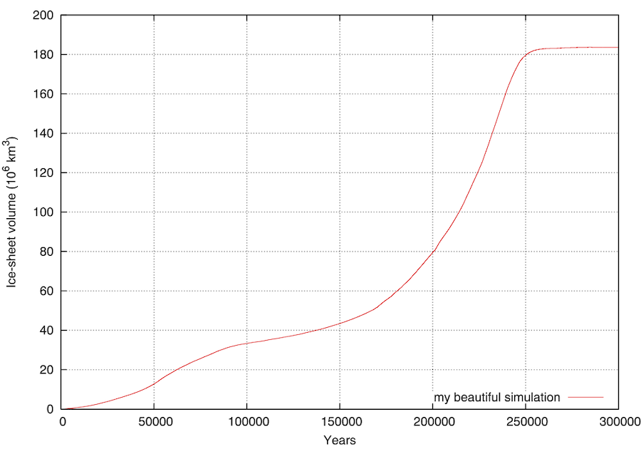
A gnuplot (!) script GRISLI/analysis/plots_GRISLI.plt is provided for that purpose. It plots key columns of the synthetic output file short*.ritz to show the time-evolution of land-ice extent and volume. In the figure below for instance, it looks like the volume took 250 kyrs to reach a steady-state.

gnuplot plots_GRISLI.plt

Interestingly, the file short*.ritz is updated during the simulation, not written at the end. Hence, it is possible to look at the evolution of land-ice volume and extent while GRISLI is running.

GRISLI volume

Of course, the same kind of figure could easily be drawn with Python if you don’t feel like using gnuplot.

If equilibrium has not been reached, the easiest solution is just to rerun the simulation from scratch for a longer duration. It is very cheap in terms of CPU time. Just be aware that every GRISLI run represents a lots of output data, hence mind your storage capacity and do not hesitate deleting useless simulations.

Looking at the results

Generating a NetCDF file

GRISLI does output a NetCDF file, e.g. 440CO06X.nc in the case of simulation GRISLI/GRISLI-version8-svn/RESULTATS/440tc_CSO_1680/440tc_CSO_1680. You can plot the output, using for instance Ferret. However, the info is stored on the GRISLI irregular grid (every grid point is a square of 40 km, rather than a grid point with regular lon-lat dimensions). The easiest way to visualize the output is to regrid the NetCDF file onto a regular grid (of your desired resolution; a grid file named Grid_LMDZ_for_GRISLI_curv2rect.txt is here provided and can be adapted as you wish):

cdo remapbil,../Grid_LMDZ_for_GRISLI_curv2rect.txt 440CO06X.nc 440CO06X_rect.nc

Plotting

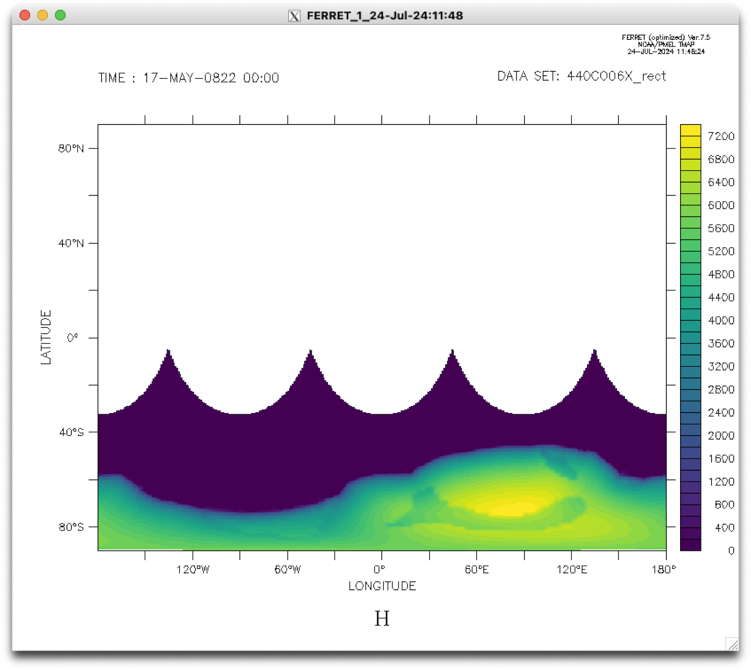
This regridded file can be inspected using Ferret (remember that GRISLI ran on a regional grid centered over the South Pole, hence the missing data over the rest of the planet).

GRISLI map Ferret

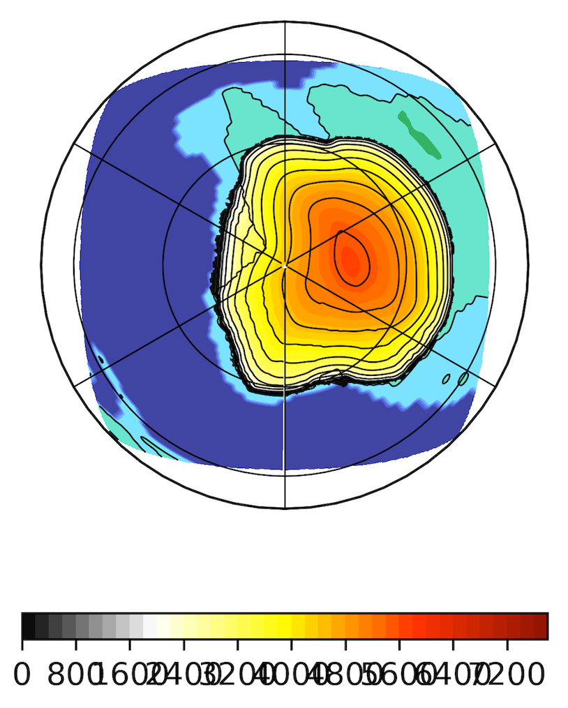
I also included a Python script that permits to easily handle projections etc.: GRISLI/analysis/map_GRISLI.py.

GRISLI map Python

Of course, it is then possible to plot the GRISLI output on top of a global paleogeographical map.

Overview of GRISLI output variables

The NetCDF is poorly formatted. As a rapid overview of the variables, here is an old file giving some key info.

     var     4       coeff.cpt       Variable_code
     Scoul   5       Surf_Pollard.cpt        Surface elevation (m) (Surf_Pollard.cpt glace_bleu.cpt gray_ice_white3.cpt)
     H       5       thick-tof.cpt   Ice thickness (m) (thick-wysiwyg3.cpt)gray_ice_white3.cpt
     B       4       socle-antar.cpt Bed elevation (m)
     MK      4       posxy.cpt       Masque
     HDOT    2       hdot.cpt        hdot (m/an)
     ICE     4       posxy.cpt       Masque glace -ICE-
    Bm      4       BM.cpt  BM-snowball.cpt        Bilan de masse (m/an)
    ACC     4       Acc-Tof.cpt             Accumulation rate (m water eq.)
    ABL     4       Abl-Tof.cpt     Ablation rate (m water eq.)
    Calv    4       Calv.cpt        Calving (reste a definir)
    DHDT    4       hdot.cpt        dhdt lagrangien (m/an)
    PDD     4       pdd.cpt         Postive Degree Day
    SIMAX   4       simax.cpt       Refreezed ice (m)
    Tann    4       Tann.cpt    Tann-snowball.cpt   Annual Surf. Temperature (<b0>C)
    Tsumm   4       Tjja.cpt        Summer Surf. Temperature (<b0>C)
    TB      2       Tbasale.cpt     Basal Temperature (<b0>C)
    phi     2       geophy.cpt      Flux geothermique (mW/m2)
    phid    2       geophy.cpt      Flux deformation (mW/m2)
    BMEL    2       bmelt-hi.cpt    Basal melting rate (m water eq.)
    UXB     2       vitesses-direction.cpt uxbar
    UYB     2       vitesses-direction.cpt uybar
    UX1/2   2       vitesses-direction.cpt uxbar 1/2
    UY1/2   2       vitesses-direction.cpt uybar 1/2
    UXSL    2       vitesses-direction.cpt ux sliding
    UYSL    2       vitesses-direction.cpt uy sliding
    FROTMX  1       frotm.cpt       frotmx (bar)
    FROTMY  1       frotm.cpt       frotmy (bar)
    TOBMX   1       tob.cpt       tobmx (bar)
    TOBMY   1       tob.cpt       tobmy (bar)
    Taushelf 2      tob.cpt contrainte moyenne shelves (bar)
    EPSXX   2       colepsfin.cpt   epsilon xx (a-1)
    EPSYY   2       colepsfin.cpt   epsilon yy (a-1)
    EPSXY   2       colepsfin.cpt   epsilon xy (a-1)
    EPS     2       colepsfin.cpt   epsilon (a-1)
    PVI     3       pvi.cpt         pvi
    HWAT    1       hwater-Tof.cpt  Basal water  hydraulic height (m)
    HDWAT   1       hwatdot.cpt     Basal water evol (m/an)
    PGX     4       pgxy-fin.cpt    Basal hydro. grad./x
    PGY     4       pgxy-fin.cpt    Basal hydro. grad./y
    KOND    1       Basal   hydro. conductivity
    NFMX    1       colnefmx.cpt    Effective Pressure (Bar)
    NFMY    1       colnefmx.cpt    Effective Pressure (Bar)
    POSX    4       posxy.cpt       Posx: 0-ground 1-stream 2-ile 3-flot
    POSY    4       posxy.cpt       Posy: 0-ground 1-stream 2-ile 3-flot
   DIVERS  4       divers.cpt      fichier colonne
-1      GS      2       Surface elevation grad. (1)
-30     UMAG    2       speed.cpt       Ice velocities (m/a)
-34     Uslid   2       speed.cpt       Sliding velocity (m/a)
-68     NEFFM   1       colnefmx.cpt    Effective Pressure (Bar)
-40     FROTM   1       frotm.cpt       Basal  drag (bar ?)
-42     TOB     1       tob.cpt         taub
-62     PGMAG   4       pgmag-fin.cpt   hydro. pressure. gradient (Pa/m)
-130    FLUX    2       flux.cpt        Ice Flux (1e2 km3.a-1)
-162    FLUXW   1       fluxwat.cpt     Basal water flux (m3.a-1)

Known issues

Colinear vectors

Sometimes GRISLI crashes because it cannot compute ice-sheet dynamics due to vector co-linearity. In this case, there is no known solution: just change your experimental setup to avoid the situation (which luckily remains rare).