A user-guide for the Fast Ocean-Atmosphere Model (FOAM) at U. Bourgogne. An ocean-atmosphere general circulation model well designed for paleoclimate investigations.

This page is not intended to replace the official FOAM user guide, but rather to provide additional / alternative material.

Information on the CCUB cluster can be found here.

Although the tutorial is built with many sections for readibility, I suggest progressing linearly since knowhow acquired in section n will sometimes be useful for section n+1.

Tutorial status: this page is finished, but the tutorial has never been tested yet. Happy to have feedbacks, and to revise and add content.

Introduction

This tutorial describes how to run the Fast Ocean Atmosphere Model (Jacob, 1997) on the linux cluster of Univ. Bourgogne (CCUB, Dijon). It should be easy to adapt to other clusters.

Please note that the FOAM source code is not freely available. The code developer, Robert Jacob, plans to upload it on GitHub soon.

The tutorial is designed as follows: baseline instructions are given for the fully coupled model (with deep ocean), and additional details are provided where applicable (in bold font) for the slab mixed-layer ocean model.

Fully coupled vs. slab model

As previously mentioned, the FOAM model can be run with a deep ocean or with a slab mixed-layer ocean.

In the fully-coupled model with deep ocean, ocean dynamics is resolved. In the slab mixed-layer version, the oceanic component consists in a 50-m deep ocean layer; ocean currents are not represented and the ocean heat transport is represented using diffusion.

The fully coupled model supposedly provides more realistic, and more mechanistic results. It requires a longer model integration time: 2000 to 3000 model years, or equivalently ca. 4 wall-clock days, to reach deep ocean thermal equilibrium.

The slab model is much lighter; it requires 50 years to reach equilibrium, or 4 wall-clock hours.

See Pohl et al. (Pohl, A., Donnadieu, Y., Le Hir, G., Buoncristiani, J.F. and Vennin, E. 2014. Effect of the Ordovician paleogeography on the (in)stability of the climate. Climate of the Past, 10, 2053–2066) for an analysis of the differences between the two model version.

Requirements

Before starting anything, you need to correctly configure your environment by loading the appropriate modules:

module purge
module load intel/2018
module load netcdf/4.6.1/openmpi/2.1.2/intel/2018
module load cdo/1.9.2/intel/2018
module load nco/4.7.7/intel/2018
module load openmpi/2.1.2/intel/2018

For comparison, here should be the result of the module list command:

Currently Loaded Modulefiles:
 1) netcdf/4.6.1/openmpi/2.1.2/intel/2018   4) intel/2018
 2) cdo/1.9.2/intel/2018                    5) openmpi/2.1.2/intel/2018
 3) nco/4.7.7/intel/2018

Remark: At some point, following cluster module updates, we will probably have to change some modules, which will require recompiling the code with these modules and loading the same version afterwards. Ideally, we’ll also have to check that results are identical.

Installing and compiling

1. Download and uncompress the model source tar xfvz foam1.5src.tar.gz (not freely available to date, see page header) in your home directory /user1/crct/zz9999zz (replace zz9999zz with your CCUB login). Then, enter the directory cd foam1.5src.

2. On the CCUB cluster, you should be all set with libraries correctly linked in the Makefile on lines 190–192:

# CCUB
NETCDF_INC= -I/soft/c7/netcdf/4.6.1/openmpi/2.1.2/intel/2018/include
NETCDF_LIB= -L/soft/c7/netcdf/4.6.1/openmpi/2.1.2/intel/2018/lib -lnetcdff -L/soft/c7/phdf5/1.8.20/openmpi/2.1.2/intel/2018/lib -pthread -L/soft/c7/netcdf/4.6.1/openmpi/2.1.2/intel/2018/lib -lnetcdf -lnetcdf
NC_LIBS = $(NETCDFC_LDFLAGS) -lnetcdff

3. Make clean to clean compiling directory from previous iterations.

4. Compile: Make foam. Everything going well, you should get an executable called foam1.5, which you should move into your home root directory (mv foam1.5 ../. or alternatively mv foam1.5 /user1/crct/zz9999zz/.

For FOAM slab: Make foamslab and then mv foam1.5.slab /user1/crct/zz9999zz/..

Now, the model is compiled and ready to run. Let’s see how to launch an experiment from a directory with all boundary and initial conditions ready. We’ll see how to create these boundary and initial conditions later.

In the following, you’ll need an ensemble of files, which are downloadable here.

Running an experiment from existing boundary and initial conditions

Directory with boundary conditions and initial conditions

In the archive that you previously downloaded (here), you will find a directory BC_300rd_T36.tar.gz containing all boundary and initial conditions required to run an random experiment at 300 Ma (taken from this dataset. Place the (uncompressed) directory in your WORKDIR (the place where you will want to run your simulations; this is a Scratchdir, although files are not automatically deleted after a given duration, as is done on other clusters) at the following location (while creating required directories): /work/crct/zz9999zz/foam/phanero/300rd/300rd_T36/BC_300rd_T36 (or another location of your choice, I propose typical paths for illustration).

Run directory

Now, let’s create the directory where the FOAM model will run. For the purpose of illustration, we will run an experiment at 2240 ppm CO2 (i.e., 8 x 280 ppm = 8 PAL pCO2, preindustrial atmospheric level) with null eccentricity. Let’s call it EcN_8X.

Create run directory

Create run directory mkdir /work/crct/zz9999zz/foam/phanero/300rd/300rd_T36/EcN_8X, enter that directory cd /work/crct/zz9999zz/foam/phanero/300rd/300rd_T36/EcN_8X and copy the content of downloaded directory run_directory there (cp run_directory/* /work/crct/zz9999zz/foam/phanero/300rd/300rd_T36/EcN_8X/.).

Now, let’s edit all requested files.

File run_params

File run_params gives the run duration and paths. In this file, replace zz9999zz with your login. All other info is OK (see below).

RESTFRQ: 360
HISTFRQ: 360
FILTPHIS: T
INITIAL: T
PREFIX: /work/crct/zz9999zz/foam/phanero/300rd/300rd_T36/EcN_8X
STORAGE: /work/crct/zz9999zz/foam/phanero/300rd/300rd_T36/EcN_8X
TIME_INV: /work/crct/zz9999zz/foam/phanero/300rd/300rd_T36/BC_300rd_T36
FINISHED: 0
RUNLNG: 720000

• RESTFRQ: the FOAM model year is 360 days.
• HISTFRQ: writing model output every year / 360 days.
• FILTPHIS and INITIAL set to T(RUE) for a new (i.e., not restarted) simulation (we filter boundary conditions).
• PREFIX: path to run directory.
• STORAGE: path to run directory.
• TIME_INV: path to boundary conditions directory.
• FINISHED: last simulated year (0 for a new simulation).
• RUNLNG: run duration, in days. 720 000 days is 2000 years (of 360 days each, see RESTFRQ).

Caution: too long a path (e.g., /work/crct/zz9999zz/foammmmmmmmm/phanero/300rd/300rd_T36/EcN_8X) will make the model crash with no clear error message. Be aware.

With the slab model, equilibrium is reached in 50 years. Just launch the model for 100 years with monthly output like this:

RESTFRQ: 360
HISTFRQ: 30
FILTPHIS: T
INITIAL: T
PREFIX: /work/crct/zz9999zz/foam/phanero/300rd/300rd_T36/EcN_8X
STORAGE: /work/crct/zz9999zz/foam/phanero/300rd/300rd_T36/EcN_8X
TIME_INV: /work/crct/zz9999zz/foam/phanero/300rd/300rd_T36/BC_300rd_T36
FINISHED: 0
RUNLNG: 36000

It should take around 4 hours for the slab simulation to run.

File atmos_params

File atmos_params defines an ensemble of parameter values, output variables and file names. More importantly, it also defines atmospheric pCO2, the solar constant and orbital configuration.

For the purpose of this turorial, you do not need to change anything.

 &CCMEXP
 PRIMARY='RELHUM',
 EXCLUDE='DC01','TS2','TS3','VD01','TS4','DTH','DTV','CMFDT','CMFDQ','DTCOND','CNVCLD','TAUGWX','QPERT','TPERT','TAUX','TAUY','UTGW','VTGW','VVPUU','NTRM','NTRN','NTRK,'NDBASE','NSBASE','NBDATE','NBSEC','MDT','MHISF','CURRENT_MSS','FIRST_MSS','INIT_MSS','TIBND_MSS','SST_MSS','OZONE_MSS','DATE','DATESEC',
 CTITLE = 'PCCM3-UW case: default',
 NCDATA = 'SEP1.R15.nc',
 BNDTI = 'tibds.R15.nc',
 BNDTVS = 'tvbds.R15.nc',
 BNDTVO = 'ozn.R15.nc',
 IRT=0,
 NSREST=3,
 NREVSN='rest',
 NSWRPS='passwd',
 NSVSN='rstrt',
 NDENS  =     1,
 NNBDAT = 000101,
 NNBSEC = 0,
 NNDBAS = 0,
 NNSBAS = 0,
 MFIfortranLT  =  1,
 DTIME  =  1800.,
 IRADSW =   -1,
 IRADLW =   -1,
 IRADAE =   -12,
 SSTCYC = .T.,
 OZNCYC = .T.,
 DIF4=2.E16,
 ACCRST = .T.,
 CO2VMR = 2240e-06,
 CH4VMR = 1.714000e-06,
 SCON = 1368e+03,
 ECCEN = 0,
 OBLIQ = 22,
 MVELP = 90,
 DAYP = 0,
 &END

• CO2VMR = 2240e-06: Atmospheric CO2 is set to 2240 ppm.
• 1368e+03: The solar constant is set to Modern (1368 W m-2). Note that this value should be changed for paleo applications.
• ECCEN = 0: Eccentricity is zero.
• OBLIQ = 22: Obliquity is 22°.
• MVELP = 90 and DAYP = 0: longitude of perihelion which has no impact here due to the null eccentricity (more info here).

File pbs.foam16p.script

File pbs.foam16p.script is a bash script permitting to submit the simulation in batch mode. For the purpose of this turorial, you do not need to change anything.

#!/bin/bash
#$ -N j300RD8
#$ -pe dmp* 32
#$ -q batch

module purge
module load intel/2018
module load netcdf/4.6.1/openmpi/2.1.2/intel/2018
module load cdo/1.9.2/intel/2018
module load nco/4.7.7/intel/2018
module load openmpi/2.1.2/intel/2018

mpirun foam1.5 run_params

#qsub pbs2

• #$ -N j300RD8: The job name, just convenient.
• #$ -pe dmp* 32 and #$ -q batch: Simulation ran in batch mode on 32 cores in parallel. More info here.

Modules are loaded (the same modules as defined at start, used also to compile the model executable), and the executable of the fully coupled model (foam1.5) is launched using the parameters found in run_params.

Linking the executable

While in the run directory, create a symbolic link (to avoid filling the disk) to the compiled executable: ln -s /user1/crct/zz9999zz/foam1.5 ..

Creating history and restart directories

While in the run directory, create the history and restart directories, for each model component (ocean, atmosphere and coupler):

• mkdir history
• mkdir history/atmos
• mkdir history/ocean
• mkdir history/coupl
• mkdir restart
• mkdir restart/atmos
• mkdir restart/ocean
• mkdir restart/coupl

Model output will be written in history (history/atmos for the atmosphere etc.), while restart files will be written in restart (restart/atmos for the atmosphere etc.).

Launching the simulation

While in the run directory, submit the job (qsub pbs.foam16p.script). You can check the run status using qstat(and will be happy at that time to see a proper run name, defined above). To abort the run, qdel job-ID, with job-IDbeing the job number (e.g. 7013515) obtained with the command qstat.

It will take approximatively 4 days to run for 2000 model years. Output is written in the history output directories (one file every 3 to 4 minutes). Useful information can be found during the run in output files om3.out.4_8.0and pccm.out.0720000.

Should the simulation crash, see section below.

Creating boundary and initial conditions

We previously ran an experiment based on a provided directory of boundary and initial conditions. It’s now time to see how to create such a directory from scratch.

Creating boundary conditions

Boundary conditions are model parameters that do not evolve during the simulation. They notably define the continental configuration, topography and bathymetry, pCO2, solar luminosity, orbital configuration etc. While some of these boundary conditions (pCO2, solar luminosity, orbital parameters) are imposed in file atmos_params (here), others (topography/bathymetry, land-sea mask, vegetation) are imposed through a series of specific files included in the directory of boundary conditions (that will be created below).

Slarti boundary conditions

Boundary conditions are created using a graphical interface named Slarti. The software Slarti.jar is included in the files you downloaded. It can be run on MacOS (open Slarti.jar) and Linux (and probably Windows, but who uses Windows?). I suggest using Slarti on your local computer for speed purposes when using the mouse.

Slarti takes in input a DEM in the form of a NetCDF raster file with 128 x 128 grid points. One example file is provided with this turorial: Topobathy_300eb_postslarti_cor.nc.

Remark: you can easily create a similar input file based e.g. on the paleoDEMS of Scotese and Wright (2018), which you may want to regrid on a 128 x 128 grid using the cdo remapbil tool (module available on the CCUB as well).

1. File/New, 128x128, R15, Bathymetry/Topography, Browse Topobathy_300eb_postslarti_cor.nc, NetCDF, no Optional Input, click OK (see screenshot below).

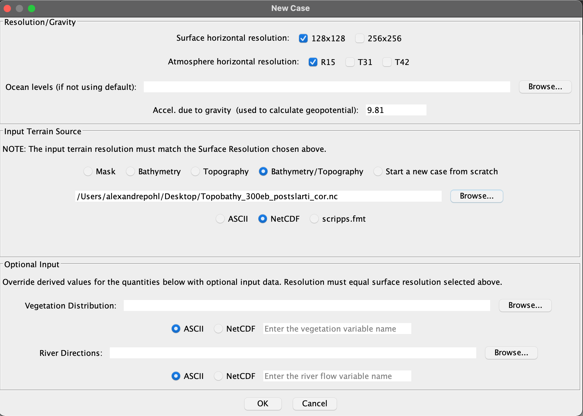
2. Please enter the bathymetry/topography variable name: TOPO in this example (you can get this info using the nco tool ncdump -h Topobathy_300eb_postslarti_cor.nc; nco module available on the CCUB as well).

3. View-Edit/Mask: You can Highlight ocean cells with no current and alter the land-sea mask manually. During this step, you have to make sure not to create any lakes, and that oceanic gateways are large enough to permit water flow (or just close them if that’s better). Don’t forget to Compare and match files and File/Save regularly, see step 4.

4. File/Save; Save for Coupled Run > OK > OK > lakes can be found at this stage, close window and Continue > OK > Next > OK > OK (you may need to enlarge the window to see the button appear), define path (e.g., /Users/username/Desktop/300rd) and OK. I suggest saving on the Desktop, since Slarti seems to have writing rights issues in some other directories.

5. View-Edit/Vegetation: Leave unchanged for a theoretical latitudinal distribution like today, or alter for deep-time periods (e.g. rocky desert in the Cambrian in the absence of land plants).

6. View-Edit/Bathymetry: Best changing level by level in step 7.

7. View-Edit/Bathymetry Level View: Level by level, make sure to avoid isolated ocean grid points where salt could accumulate, which would make the model drift and ultimately crash (see section below).

8. View-Edit/Topography: Topography can be altered here, but keep in mind that the atmosphere will see a lower-resolution version (only shown when saving). What you see here is the topography seen by the coupler.

9. View-Edit/River flow: define the water routing manually (by imposing flow directions: North, North-East, East, SE, S, etc.), while making sure to avoid creating lakes. Please remember to Compare and match files when switching from one window to another one. For instance, changing the topography will automatically alter the river flow. Be aware of this. At any time, you can manually List river flow lakes. No lakes should be found in the final boundary conditions. If lakes are found, you have to get rid of them.

10. At any time, you can save your boundary conditions in their current state (see previous step 4) and resume editing later. Just open Slarti and File/Open the .case file included in your directory of saved boundary conditions.

The slab model has no routing and lakes can exist. However, it means that you will not be able to run the fully coupled model using the same directory of boundary conditions. I suggest always preparing clean boundary conditions for the coupled model, even if you wanna run the slab version.

Importantly, you can use the (uncompressed) directory of boundary conditions provided with this tutorial (BC_300rd_T36) to look at the expected Slarti output. To that purpose, open Slarti and File/Open, find uncompressed directory BC_300rd_T36 and open file 300rd.case.

[optional] Building the resulting topography/bathymetry NetCDF file.

With Ferret, run script UTIL/TopoBathyBuild_Cor.jnl, using your Slarti directory file in input, to generate the 2D topography/bathymetry NetCDF file with the paleogeography created in Slarti.

This is an optional step. This file is not needed to run the model.

Gathering required files

Let’s gather all required files in a directory (just as you previously used directory BC_300rd_T36, uncompressed from BC_300rd_T36.tar.gz).

1. Create a new directory /work/crct/zz9999zz/foam/phanero/300rd/300rd_T36/BC_300rd_T37. Name is arbitrary here, do not search for any meaning.

2. Copy a series of requested files available in the files you previously downloaded: cp TOADD/* /work/crct/zz9999zz/foam/phanero/300rd/300rd_T36/BC_300rd_T37/.

3. Copy the Slarti output files. These files should normally now be saved on your local computer. Use scp to send them on the cluster. scp 300rd/* zz9999zz@krenek2002.u-bourgogne.fr:/work/crct/zz9999zz/foam/phanero/300rd/300rd_T36/BC_300rd_T37/..

4. Enter the directory cd /work/crct/zz9999zz/foam/phanero/300rd/300rd_T36/BC_300rd_T37/ and rename 2 files: mv tibds.R15.* tibds.R15.ncand mv initial.R15.* SEP1.R15.nc.

Now, your boundary conditions are ready. In order to test them in this tutorial, we can simply adapt the paths used in the EcN_8X experiment that we previously set up. To that purpose, just edit file run_params: TIME_INV should new read /work/crct/zz9999zz/foam/phanero/300rd/300rd_T36/BC_300rd_T37.

Make sure (with qstat) that the simulation is not currently running (or stop it using qdel; otherwise, both simulations will run simultaneously and overwrite output files) and launch it with qsub pbs.foam16p.script.

Creating initial conditions

Initial conditions define model ‘starting’ conditions, for instance ocean temperature and salinity, which are expected to change during the model run.

You will be interested in 2 specific files defining ocean initial salinity and temperature.

With the slab model, ocean dynamics are not resolved. Please ignore this paragraph on the model initial conditions

Field of initial salinity

The default field of initial salinity is Modern and defined in file BC_300rd_T37/om3.salt24 (previous copied from the TOADD directory).

For paleo applications, you will be interested in starting with a globally uniform ocean salinity field. Such file, with global salinity of 35 permil, is found in the files your previously downloaded, here: UTIL/om3.salt35. To use it:

1. In your directory of boundary conditions (/work/crct/zz9999zz/foam/phanero/300rd/300rd_T36/BC_300rd_T37), delete default file: rm om3.salt24.

2. Copy desired file: cp UTIL/om3.salt35 /work/crct/zz9999zz/foam/phanero/300rd/300rd_T36/BC_300rd_T37/..

3. Create symbolic link: ln -s om3.salt35 om3.salt24 (since FOAM expects to find a file named om3.salt24). Actually, you could just mv om3.salt35 om3.salt24 or cp om3.salt35 om3.salt24, but the symbolic link permits keeping track of the file used.

Field of initial ocean temperature

Similarly, the default field of initial temperature is Modern and defined in file BC_300rd_T37/om3.temp24 and you can replace it with any file found in directory UTIL (e.g., om3.temp24_20_5_1_1). These files are all named using the same pattern: om3.temp24_, followed by: equatorial surface temperature, equatorial thermocline temperature, sea-bottom temperature and polar temperature (both supposed to be identical due to deep-water formation at the poles).

I suggest to use a warm initial ocean (around 3 degrees warmer than expected equilibrium temperature) in order to ensure intense oceanic convection and a rapid deep-ocean temperature equilibrium.

The FOAM model climatic sensitivity being around 3°C, I provide initial temperature files every ~3 degrees. You can also create your own intial temperature fields using the Matlab and Python routines provided in directory UTIL/NEWEQ.

1. First run the Matlab script raw_om3_temp24.m to generate a NetCDF file with the expected temperature data.

2. Then, run the Python script AP_theoretical_nc_to_om3.py to convert the NetCDF into a binary file om3.temp24 that can be read by FOAM.

Checking for equilibrium and generating output files

Checking for equilibrium

After 2000 model years of simulation, you will be interested in checking for deep-ocean thermal equilibrium. To that purpose:

1. Generate time series by copying file UTIL/EvolBis.py into your history/ocean model output directory and running it with python EvolBis.py. It will take a while and output a file named history.ocean.evol.an001a2000.nc.

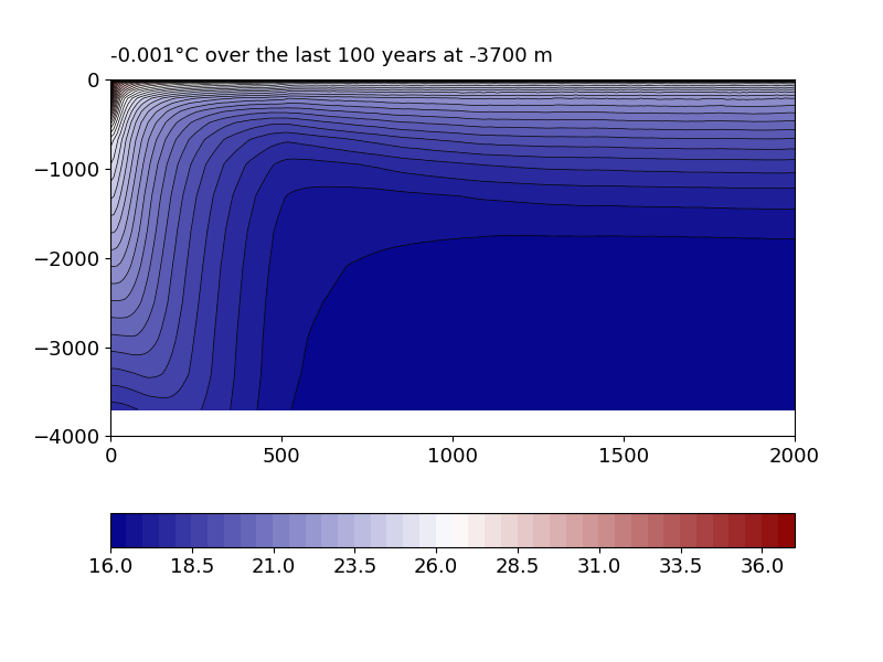
2. Plot the time-evolution of temperature over the water column using the script UTIL/checkevol.py (which looks for the file that you previously created, history.ocean.evol.an001a2000.nc).

You will get a figure like the one below, also calculating the deep-ocean temperature drift over the last 100 years. The latter should be very small.

If equilibrium has not been reached after 2000 model years, you have several options:

1. Give up and go and play outside.

2. Restart the simulation for another, say, 1000 years. To do that, just edit file run_params. FILTPHIS and INITIAL should be set to F, FINISHED to 2000 years and RUNLNG to 1000 additional years:

RESTFRQ: 360
HISTFRQ: 360
FILTPHIS: F
INITIAL: F
PREFIX: /work/crct/zz9999zz/foam/phanero/300rd/300rd_T36/EcN_8X
STORAGE: /work/crct/zz9999zz/foam/phanero/300rd/300rd_T36/EcN_8X
TIME_INV: /work/crct/zz9999zz/foam/phanero/300rd/300rd_T36/BC_300rd_T37
FINISHED: 720000
RUNLNG: 360000

3. If you think the issue comes from inadequate initial conditions (e.g., too warm an initial ocean), you can use this knowledge to run a new simulation with better-suited initial conditions (just change the om3.temp24 file and start the simulation from scratch; previous output files with be overwritten).

With the slab model, you can check for equilibrium by running UTIL/EvolSlab.py in your history/atmos model output folder and subsequently using the output time-series NetCDF file to plot the time-evolution of atmospheric surface temperature TS1 (but it’s not even necessary, the slab model will reach equilibrium in 50 years).

Generating output files

As any GCM, FOAM displays some internal variability. In order to get ‘climatology’ files, we will have to calculate mean monthly values over the last 30–50 years – personally and below, I use 50 years. It will require 2 steps:

Running the model with monthly output

Edit file run_params (or create a new one, named for instance run2) as follows:

RESTFRQ: 360
HISTFRQ: 30
FILTPHIS: F
INITIAL: F
PREFIX: /work/crct/zz9999zz/foam/phanero/300rd/300rd_T36/EcN_8X
STORAGE: /work/crct/zz9999zz/foam/phanero/300rd/300rd_T36/EcN_8X
TIME_INV: /work/crct/zz9999zz/foam/phanero/300rd/300rd_T36/BC_300rd_T37
FINISHED: 720000
RUNLNG: 18000

• HISTFRQ: set to 30 for monthly output (every 30 days).
• FILTPHIS and INITIAL: set to F for a restart.
• FINISHED: restarting from year 2000.
• RUNLNG: 18 000 days (50 years of 360 days each).

Then, submit pbs.foam16p.script (if you created a new run2 file, you have to make sure that pbs.foam16p.script, or a newly-created pbs2 file, calls the right parameters, here run2). It will take around 4 hours to run for 50 years.

Important remark: With the CCUB, some restart/atmos files are not named properly. Check for any issue before restarting an experiment. Indeed, each atmospheric restart should consist in two files (here for year 2000) restart.atmos.0720000.A and restart.atmos.0720000. Typically, restart.atmos.0720000 will be incorrectly named r2001, or similar. Just mv r2001 restart.atmos.0720000, or ln -s r2001 restart.atmos.0720000.

With the slab model, you previously ran the model for 100 years with monthly output. No need to run an additional job, then. Climatology will be calculated over the last 50 years, see below.

Generating climatology files

We generate climatology files for each model component: ocean, atmosphere and coupler, by calculating monthly means over the last 50 model years.

1. Once the monthly output generated, copy the python script UTIL/NewMois.py into your ocean output directory (cp UTIL/NewMois.py /work/crct/zz9999zz/foam/phanero/300rd/300rd_T36/EcN_8X/history/ocean), check that everything is OK (see code and explanations below) and run the script (python NewMois.py).

    prefix = 'history.ocean.'
    year = 2000
    nyears = 50
    endname ='300rd_1368W_EccN_ocean_2240ppm.nc'
   

   • prefix: to be adjusted, ocean, atmos or coupl.
   • year: duration of the spinup (long run with annual output), here 2000 years.
   • nyears: duration of the short run with monthly output, here 50 years.
   • endname: name of the output climatology file; to be adjusted, including ocean, atmos or coupl.

2. Then, cp NewMois.py ../atmos/., cd ../atmos/. and edit NewMois.py: prefix = 'history.atmos.' and endname ='300rd_1368W_EccN_atmos_2240ppm.nc'. Run the script.

3. Do the same for the coupler (cp NewMois.py ../coupl/. etc.).

As a result, the output of each FOAM experiment is presented in the form of 3 files, each associated with a given model component, and each containing specific variables (oceanic variables for the ocean output file etc.):

• 300rd_1368W_EccN_ocean_2240ppm.nc;
• 300rd_1368W_EccN_atmos_2240ppm.nc;
• 300rd_1368W_EccN_coupl_2240ppm.nc.

With the slab model, use NewMoisSlab.py and skip step #1 (there is no oceanic output). As a result, the output of each FOAM-slab experiment is presented in the form of only 2 (instead of 3) files.

Debugging

Different cases:

Nothing bad happened

Sometimes, the model just crashes without known reason, probably due to issues with the cluster. In that case, just check that restart/atmos files are well named (see Known Issues below) and restart the experiment (see e.g. this previous section for how to restart an experiment).

Timestep issue

Sometimes, the model crashes and an error like point IJ out of bounds shows up in the error files (om3.out.4_8.0 or pccm.out.0720000, I can’t remember). It means that you’re not respecting the CFL criteria. In short, your model particle traveled over a distance longer than a grid point during the model integration time (time step).

In order to solve this issue, you can temporarily decrease the time step. In atmos_params, change the following:

• DTIME = 1200., (instead of 1800);
• DIF4=1.E16, (instead of 2.E16).

Run the model for a few time steps and then revert back to the standard values.

This workaround is useful in the presence of a sea-ice front located at the mid latitudes (which generates very strong temperature contrasts and winds/currents) or when simulating a very, very warm climate.

Salt anomaly

Another usual issue, which will probably show up in your first fully coupled model simulations due to small mistakes in Slarti.

An isolated ocean point in the land-sea mask, or a deep ocean point surrounded by shallower ocean grid points, or a very flat and relatively shallow bathymetry at the tropics (with negative P-E balance) or at the high latitudes (with sea-ice formation and associated salt fluxes), will lead to the excessive accumulation of salt and make the model crash.

This issue can generally be spotted by plotting the maximum salinity over the whole water column and determining where salinity exceeds reasonable values, and corrected by going back to Slarti, correcting the boundary conditions locally, and running a new simulations using these corrected boundary conditions.

Known issues

Restart files

With the CCUB, some restart/atmos files are not named properly, which makes the model crash upon restart.

Check for any issue before restarting an experiment. Indeed, each atmospheric restart should consist in two files (here for year 2000) restart.atmos.0720000.A and restart.atmos.0720000. Typically, restart.atmos.0720000 will be incorrectly named r2001, or similar. Just mv r2001 restart.atmos.0720000, or ln -s r2001 restart.atmos.0720000.

Too long a name

Too long a path (e.g., /work/crct/zz9999zz/foammmmmmmmm/phanero/300rd/300rd_T36/EcN_8X) will make the model crash with no explicit error message. It even happened that a given path name made the model crash… for unknown reasons except this given name?

Looking at the model output

The FOAM model output consists in standard, self-describing and cross-platform NetCDF files. You can use various tools to open such files and generate figures and diagnostics. Here is a short selection:

1. The legacy software used to treat the FOAM output is the very convenient and simple scripting language Ferret, which can be installed on Linux clusters or even locally, including on MacOS. PyFerret is just an upgrade but remains largely similar.

2. A more complex but way more powerful tool is Python.

3. You can also think about R (free), Matlab (expensive) and others (Scilab, NCL etc.).

4. If you’re looking for a graphical interface, Panoply could do the job.

5. A more complex but more powerful tool with graphical interface is a GIS, such as QGIS (free) or ArcGIS (very expensive).

References using FOAM

Here is a (non-exhaustive) list of references illustrating the use of FOAM:

• Chaboureau, A.C., Donnadieu, Y., Sepulchre, P., Robin, C., Guillocheau, F. and Rohais, S. 2012. The Aptian evaporites of the South Atlantic: A climatic paradox? Climate of the Past, 8, 1047–1058, https://doi.org/10.5194/cp-8-1047-2012.
• Dal Corso, J., Mills, B.J.W., Chu, D., Newton, R.J. and Song, H. 2022. Background Earth system state amplified Carnian (Late Triassic) environmental changes. Earth and Planetary Science Letters, 578, 117321, https://doi.org/10.1016/j.epsl.2021.117321.
• Donnadieu, Y., Pucéat, E., Moiroud, M., Guillocheau, F. and Deconinck, J.F. 2016. A better-ventilated ocean triggered by Late Cretaceous changes in continental configuration. Nature Communications, 7, 10316, https://doi.org/10.1038/ncomms10316.
• Goddéris, Y., Donnadieu, Y., Le Hir, G., Lefebvre, V. and Nardin, E. 2014. The role of palaeogeography in the Phanerozoic history of atmospheric CO2 and climate. Earth-Science Reviews, 128, 122–138, https://doi.org/10.1016/j.earscirev.2013.11.004.
• Hearing, T.W., Harvey, T.H.P., et al. 2018. An early Cambrian greenhouse climate. Science Advances, 4, eaar5690, https://doi.org/10.1126/sciadv.aar5690.
• Ladant, J.-B. and Donnadieu, Y. 2016. Palaeogeographic regulation of glacial events during the Cretaceous supergreenhouse. Nature communications, 7, 12771.
• Le Hir, G., Donnadieu, Y., et al. 2009. The snowball Earth aftermath: Exploring the limits of continental weathering processes. Earth and Planetary Science Letters, 277, 453–463, https://doi.org/10.1016/j.epsl.2008.11.010.
• Le Hir, G., Donnadieu, Y., Goddéris, Y., Meyer-Berthaud, B., Ramstein, G. and Blakey, R.C. 2011. The climate change caused by the land plant invasion in the Devonian. Earth and Planetary Science Letters, 310, 203–212, https://doi.org/10.1016/j.epsl.2011.08.042.
• Lee, S.-Y. and Poulsen, C.J. 2006. Sea ice control of Plio–Pleistocene tropical Pacific climate evolution. Earth and Planetary Science Letters, 248, 253–262.
• Licht, A., van Cappelle, M., et al. 2014. Asian monsoons in a late Eocene greenhouse world. Nature, 513, 501–506.
• ills, B.J.W., Donnadieu, Y. and Goddéris, Y. 2021. Spatial continuous integration of Phanerozoic global biogeochemistry and climate. Gondwana Research, https://doi.org/10.1016/j.gr.2021.02.011.
• Nardin, E., Goddéris, Y., Donnadieu, Y., Le Hir, G., Blakey, R.C., Pucéat, E. and Aretz, M. 2011. Modeling the early Paleozoic long-term climatic trend. Bulletin of the Geological Society of America, 123, 1181–1192, https://doi.org/10.1130/B30364.1.
• Pohl, A., Donnadieu, Y., Le Hir, G., Buoncristiani, J.F. and Vennin, E. 2014. Effect of the Ordovician paleogeography on the (in)stability of the climate. Climate of the Past, 10, 2053–2066.
• Pohl, A., Donnadieu, Y., et al. 2020. Carbonate platform production during the Cretaceous. GSA Bulletin, 132, 2606–2610, https://doi.org/10.1130/B35680.1.
• Pohl, A., Lu, Z., et al. 2021. Vertical decoupling in Late Ordovician anoxia due to reorganization of ocean circulation. Nature Geoscience, 14, https://doi.org/10.1038/s41561-021-00843-9.
• Poulsen, C.J., Pierrehumbert, R.T. and Jacob, R.L. 2001. Impact of ocean dynamics on the simulation of the neoprotozoic ‘snowball earth’. Geophysical Research Letters, 28, 1575–1578, https://doi.org/10.1029/2000GL012058.
• Poulsen, C.J., Gendaszek, A.S. and Jacob, R.L. 2003. Did the rifting of the Atlantic Ocean cause the Cretaceous thermal maximum? Geology, 31, 115–118.
• Saupe, E.., Qiao, H.., et al. 2019. Extinction intensity during Ordovician and Cenozoic glaciations explained by cooling and palaeogeography. Nature Geoscience, 13, 65–70, https://doi.org/10.1038/s41561-019-0504-6.
• Wong Hearing, T.W., Pohl, A., et al. 2021. Quantitative comparison of geological data and model simulations constrains early Cambrian geography and climate. Nature Communications, 12, 3868, https://doi.org/10.1038/s41467-021-24141-5.
• Zacaï, A., Monnet, C., Pohl, A., Beaugrand, G., Mullins, G., Kroeck, D.M. and Servais, T. 2021. Truncated bimodal latitudinal diversity gradient in early Paleozoic phytoplankton. Science Advances, 7, eabd6709, https://doi.org/10.1126/sciadv.abd6709.